Google announced Meridian in 2024, made it generally available in January 2025 and released version 2.0 in September 2026. It handles the hard maths in a Bayesian marketing mix model (MMM): sampling, convergence checks, adstock, saturation and budget optimisation. What it leaves to you is what to feed it and how far to trust what comes out, and that's where most of the work is.
This is the whole build in the order I run it, with the code. Every step maps to a file in meridian-mmm-toolkit, an MIT-licensed repo extracted from a production model. The worked examples come from the toolkit's synthetic brand, which has known true returns, so you can see where the model gets close to the truth and where it doesn't. Put together, the steps make a measurement system you can rerun every quarter, rather than a one-off model.
Before you start
MMM is the oversight layer: it estimates what paid media caused, a question platform reporting isn't built to answer (L/004 makes that case). It complements the signal layer rather than replacing it. If Enhanced Conversions and Meta's Conversions API (CAPI) are still leaking (L/003), fix that first.
Google's rule of thumb is at least two years of weekly data for a model by market and three for a national one, covering spend, impressions and sales. It's a starting point: the real requirement depends on how many channels you model and how much their spend varies, and more years give the seasonal shape more than one peak to learn from. You'll also need Python: Meridian 2.1 supports 3.11 to 3.13, and the toolkit is tested on 3.12 and 3.13. The code is written for Meridian 2.x, and the toolkit pins 2.1.0. And it helps a great deal to have the data in a warehouse already (L/006): with clean order and ad tables in BigQuery, the first fit runs on the first day and a validated model takes days rather than weeks.
Try it on the synthetic brand before touching real data. The smoke fit takes about a minute and only proves the plumbing works; --sampling standard takes 5 to 15 minutes on a laptop and gives numbers worth reading.
git clone https://github.com/performify-github/meridian-mmm-toolkit.git
cd meridian-mmm-toolkit
python3.12 -m venv .venv && source .venv/bin/activate
pip install -r requirements.txt

python3 mmm/synthetic.py --config example/mmm.yaml        # a fake brand with known true returns
python3 mmm/run_mmm.py --config example/mmm.yaml check --data
python3 mmm/run_mmm.py --config example/mmm.yaml local --sampling smoke --run-id demo
python3 mmm/readout.py --config example/mmm.yaml --main demo --local-dir runs --out readout
What Meridian actually does
Meridian is a Bayesian hierarchical model. Each channel contributes to the outcome through a direct effect, carry-over from earlier spend (adstock) and diminishing returns at higher spend (saturation), alongside a baseline and the things that move sales but aren't ads. Saturation is a Hill curve, which can be S-shaped: returns can build before they diminish, so the number that matters for a budget decision is the return on the next pound, not where the curve looks flat. In a geo model, each market gets its own level and the channel effects are estimated across all markets at once, which helps when one market has little data.
The baseline is what would have sold with no paid media at all. It has a level for each market, a trend that can bend at the knots (step 4), yearly seasonality, and the controls you give it: discounts, sale weeks, holidays and the demand series in step 2. Errors in the baseline land on the channels, which is why steps 2, 4 and 5 are as much about the baseline as the channels.
The Bayesian part matters. Rather than one estimate per parameter, Meridian returns a posterior distribution: everything the data supports, given the priors. That is what lets you say "paid search contribution is £480k plus or minus £90k at a 90% credible interval" rather than the false precision of "£487,213".
Under the hood it samples with Hamiltonian Monte Carlo (the No-U-Turn Sampler). A weekly model with four markets, four channels and about 200 weeks fits in 10 to 15 minutes on eight CPU cores, produces hundreds of posterior draws per parameter, and reports convergence (R-hat) and a model review you check before believing anything.
Meridian isn't the only option. PyMC-Marketing is another Bayesian framework, and Meta's Robyn takes a regularised-regression approach. Meridian has its own opinions too (a hierarchical structure, the NUTS sampler, Hill saturation). I build on it because it's production-grade, well documented and maintained by Google, which makes it easy to stand behind with a client. Most of the steps below apply whichever you use.
Meridian can also model video and reach channels from reach and frequency rather than impressions, and then optimise how often people see an ad as well as how much is spent. The toolkit uses impressions. Reach doesn't add up across weeks or markets, so it has to be pulled from each platform at exactly the model's grain, market by week, and that's worth doing once video and reach are a large share of the budget.
Step 1: one row per market per week
The model reads one table: one row per market per week, every market in every week. It holds what you're explaining (orders, with revenue so returns read in money), spend and impressions per channel, a demand series (step 2), and the other things that move sales but aren't ads, such as discount depth and sale weeks. The toolkit adds calendar flags (Black Friday, Christmas, New Year, Easter) and population itself.
week_start, geo, orders, revenue,
spend_google_convert, impressions_google_convert,
spend_google_upper,   impressions_google_upper,
spend_meta_convert,   impressions_meta_convert,
spend_meta_upper,     impressions_meta_upper,
brand_search_clicks, brand_trends_index,   # demand (step 2)
discount_depth, sale_campaign_live          # other controls
- Group campaigns by platform and funnel role, not by campaign name: Google conversion (Performance Max, Shopping, non-brand search), Google upper funnel (YouTube, Demand Gen), Meta conversion, Meta reach. Four to six channels is plenty.
sql_views.pybuilds the table in BigQuery from an ads table and an orders table using ordered rules in the config, and writes a QA query listing every campaign and the channel it landed in. Read that list once, by eye. - A new channel joins the group that does the same job. With a few months of spend, mostly in weeks a sibling channel also ran, the model can't separate the two, and a channel of its own would just return its prior. Pool it with the channel that does the same job at a similar cost (a new social platform's reach campaigns with the existing reach group, say). Give it its own channel once it has about six months of spend that moves on its own; the prior check in step 3 says when it's ready.
- Brand search is a control, not a channel. It captures demand rather than creating it.
- Compute first orders yourself if you model new customers. A "returning customer" flag set on the customer rather than the order marks every order from anyone who has ever bought twice, the first one included.
- Every date is a week start. Meridian's time points are week starts, so holdout and optimisation dates must be too.
check --datacatches it, along with missing weeks and spend that mapped to no channel or no market.
Step 2: control for demand
This step has the biggest effect on whether the channel results can be trusted, and Meridian's review doesn't check for it. Some channels spend more when demand already exists: brand search, the brand Shopping ads inside Performance Max (PMax), retargeting, Advantage+-style conversion campaigns. Their spend rises in the weeks people were going to buy anyway, and a model that can't see that demand gives them the credit.
The toolkit's synthetic brand is built with that trap. Its conversion channels spend more when demand is high, and its brand-search clicks are partly caused by its video and reach ads. Because the data is made up, the true return of every channel is known:
| Channel | True return per £1 | No demand control | Brand clicks + Google Trends | Google Trends only |
|---|---|---|---|---|
| Google PMax / Shopping | 1.80 | 3.30 (2.20-4.78) ✗ | 2.29 (1.40-3.71) ✓ | 2.43 (1.50-3.77) ✓ |
| Meta conversion | 1.30 | 2.62 (1.90-3.62) ✗ | 1.85 (1.25-2.85) ✓ | 1.93 (1.29-2.97) ✓ |
| Google YouTube / Demand Gen | 1.10 | 0.59 (0.27-1.12) ✓ | 0.49 (0.22-0.95) ✗ | 0.85 (0.38-1.43) ✓ |
| Meta reach | 0.70 | 0.78 (0.34-1.38) ✓ | 0.38 (0.17-0.71) ✓ | 0.60 (0.27-1.05) ✓ |
Median and 90% range; ✓ means the true value is inside the range. With no demand control, both conversion channels come out at about double their true return, with ranges that miss the truth. That run converged and passed Meridian's review with nothing flagged. The full outputs, including Meridian's own HTML report, are in the toolkit's example/outputs folder.
The same mistake shows up in the baseline. Paid media truly drives 20% of the synthetic brand's orders. With the demand control, the model puts it at 21% (16% to 28%); without one, at 31% (25% to 38%), so the ads get credit for about half as many orders again as they caused.
Two series work as the control, entered in the baseline per market:
- Brand-search clicks, the most direct measure of people looking for the brand.
- Google Trends interest in the brand's topic, per country, using the language-independent topic rather than a keyword, and weighted by sales share where a market spans several countries.
trends.pyfetches and loads it. It's less tied to your own ad delivery than clicks are, though not fully independent of it: upper-funnel ads can raise brand searches too. In the synthetic brand it's built to be independent; on real data it can take some upper-funnel credit, but less than clicks do.
demand_controls:
  series:
    clicks: brand_search_clicks
    trends: brand_trends_index          # Google Trends, brand topic (mmm/trends.py)
    proxy: brand_search_eligible_impressions   # weak: drops to 0 when brand search pauses
  default: clicks+trends
The trade-off shows in the table: because brand clicks are partly caused by the upper funnel, controlling for them takes some of video's and reach's credit away. The Trends-only run recovers every channel here. On real data you don't know the truth, so run both and report the range. A weaker proxy, brand impressions divided by impression share, is too noisy and falls to zero whenever a brand campaign pauses.
Two options go further. Meridian 2.0's full-funnel framework adds branded search volume as a brand signal, so upper-funnel ads can be credited with the brand searches they create; the toolkit doesn't use it yet, and on 2.x it's worth running alongside the control approach. And if you can get Google Query Volume through Google's MMM Data Platform, Meridian's documentation recommends it as a control for paid search; Trends is the public alternative.
On a real account, the symptom is a lower-funnel channel whose return lands above the platform's own reported ROAS and barely moves when you halve its prior. Before believing it, read the ad account. Performance Max brand exclusions cover Search, Shopping and YouTube search by default, but there's an option to keep Shopping ads serving on excluded brand terms, so check which the campaign uses. Its search-term insights show how much of its value comes from brand searches. And a brand search campaign that's capped by budget pushes brand queries into PMax. Add or strengthen the demand control; don't tune the prior to hide it. L/022 is a production build where exactly this happened: the first fits credited PMax with double Google's own figure.
Step 3: priors you can defend
Priors are your best estimate of each channel's return before the model sees the data. They come from published benchmarks, past engagements in similar categories and the brand's own tests. The toolkit keeps them in a file, one row per channel, with a source on every row:
channel,roi_low,roi_high,mass,status,source
google_convert,0.5,4.0,0.9,EXAMPLE,"benchmarks for paid search / Shopping, top end near the platform's ROAS"
google_upper,0.3,3.0,0.9,EXAMPLE,"online video benchmarks and incrementality studies"
meta_convert,0.5,3.5,0.9,EXAMPLE,"paid social benchmarks, top end near Meta's reported ROAS"
Each range becomes a LogNormal ROI prior holding 90% of its mass between the two values:
_ln = prior_distribution.lognormal_dist_from_range(
    pri["roi_low"].tolist(), pri["roi_high"].tolist(), mass_percent=0.9)
roi_prior = backend.tfd.LogNormal(_ln.loc, _ln.scale, name=constants.ROI_M)
spec_kwargs = dict(prior=prior_distribution.PriorDistribution(roi_m=roi_prior),
                   max_lag=8, holdout=holdout)
- Use the platform's own reported ROAS as a plausibility check for the lower funnel. Setting the top of the range near it means a channel has to earn a higher return from the data. It isn't a hard ceiling: about 5% of the prior still sits above the top of its range, and attribution windows and offline sales can legitimately put the true return above or below the platform's figure.
- Keep upper-funnel ranges wide. A short-term, online-only model sees little of video and reach, so their posteriors lean on the prior.
- After the fit, compare each posterior with its prior. If they barely differ, the data had little to say: the number is a benchmark rather than evidence, and it belongs on the test list (see the end of this guide).
priors.csv (grey) against where the model ended up after the data (blue: median and 90% range), with the true return marked. The data narrowed every range, the conversion channels' most. The readout draws this for every fit, and flags a channel whose range barely narrowed (mostly the benchmark: test it) or that landed outside its prior's range (check for demand leaking in).A benchmark is where a prior starts; a test is better. The toolkit takes lift-test results in a second file, one row per test: the channel, the test's dates, the return per £1 it measured with its standard error, and the spend it covered. Each result replaces that channel's benchmark prior.
channel,start,end,estimate,standard_error,kpi_type,spend,status,source
google_convert,2024-05-06,2024-06-30,1.763,0.353,revenue,7409.21,SIMULATED,"brand on/off, one market, eight weeks"
Meridian adjusts each test before using it, and the adjustment can be large. It widens the test's uncertainty when its daily spend is far from the channel's usual level, when it's short and when it's old. The synthetic brand's simulated test above ran in one market of four and ended 18 months before the data does. It read the true return almost exactly and still went in with its standard error more than doubled, from 0.35 to 0.79. In the run with no demand control it moved PMax from 3.30 only to 3.02, against a true 1.80. A test refines a model; it doesn't rescue one that's missing its demand control. Run tests close to the refit, at a realistic share of the channel's spend.
Flat priors "to let the data speak" sound neutral, but they aren't. On a few years of data where channels rise and fall together, the data alone often can't separate their effects, so the model can fit the past well and still say little that's reliable about each channel. A good MMM report shows its priors and where they came from.
Step 4: knots and Fourier terms
model:
  max_lag: 8        # an ad's effect can carry on for up to 8 weeks
  knots: monthly    # where the baseline can bend: monthly | quarterly | aks | a number
  fourier: 2        # smooth yearly waves for the seasonal peak
- Always set knots in a geo model. Left unset, every week gets its own baseline, which swallows any campaign that ran in all markets at once. Roughly monthly is a good default.
- Add annual Fourier terms as controls for the seasonal peak. Without them, a peak the model hasn't seen (step 5) has nothing to be predicted from.
- One seasonal curve is shared across markets, so it follows the biggest market's peak. A market whose year peaks somewhere else (spring rather than Christmas, say) gets misfitted there. Check the error per market, not just overall, and give that market its own seasonal controls.
- How markets are scaled against each other is an assumption too. Scaling by population or by orders can move credit between the two big conversion channels in the main market. Run both and report the split as a range if it moves.
Step 5: hide weeks the model has to predict
Any flexible model fits the weeks it was shown. The test is whether it predicts weeks it wasn't. Three holdouts, from easy to hard:
holdouts:
  random:        {type: random, ratio: 0.1}           # a random 10% of market-weeks
  peak_one_geo:  {type: geo_dates, geos: [UK], start: "2024-10-07", end: "2024-12-23"}
  peak_all_geos: {type: dates, start: "2024-10-07", end: "2024-12-23"}
| Holdout (synthetic brand) | R² on hidden weeks | Converged |
|---|---|---|
| A random 10% of weeks | 0.99 | yes |
| Q4 2024 hidden in one market | 0.93 | yes |
| Q4 2024 hidden in every market | 0.42 | no (R-hat 2.1) |
The last one is the hardest test: every knot in those weeks has no data in any market, so the peak has to come from the other years. It often fails, and a run that hasn't converged isn't presented; read it as "the peak can't be predicted from the other weeks alone". The one-market version, Meridian's GeoHoldoutSpec, is the fairer test, because the other markets keep anchoring the shared baseline. Choose the model's settings on all three holdouts, not on how well it fits the weeks it has seen.
Step 6: change one thing at a time
A fit costs about 15 minutes and pennies in the cloud, so report a model as a grid of them, each changing one assumption:
--priors-scale 0.5            --run-id sens{date}-priors-x0.5
--priors-scale 2              --run-id sens{date}-priors-x2
--demand-control trends       --run-id sens{date}-trends-only
--no-demand-control           --run-id sens{date}-no-demand-control
--knots quarterly             --run-id sens{date}-quarterly-knots
--fourier 0                   --run-id sens{date}-no-fourier
--kpi new_customers           --run-id sens{date}-new-customers
--experiments experiments.csv --run-id sens{date}-lift-test
run_mmm.py queue keeps a set number of fits running at once and resubmits any that hit a quota. Then sort the results into two lists: what held in every run, and what moved. Only the first kind can bear a budget decision. Quote the second as ranges, and put it on the test list.
Step 7: fit, then read the review properly
python3 mmm/run_mmm.py --config brand/mmm.yaml local  --sampling standard --run-id main-local
python3 mmm/run_mmm.py --config brand/mmm.yaml submit --sampling standard --run-id main-cloud
python3 mmm/run_mmm.py --config brand/mmm.yaml status main-cloud
Each run writes a summary (convergence, the review, holdout accuracy, and ROI, marginal ROI and share per channel with 90% ranges), Meridian's own HTML report, the budget scenarios and the saved model. Read them in this order:
- Convergence. R-hat below 1.1 everywhere; don't present a run above 1.2. A run that hasn't converged can still produce plausible-looking numbers, so check this first.
- The review. All of Meridian's checks should pass, but a pass doesn't mean the answer is right: the no-demand-control run in step 2 passed too.
- Marginal ROI before ROI. ROI is the average over the period; the return on the next £1 is the budget number.
- The platform's figures, like for like. Platform ROAS is often VAT-inclusive, click-window based and overlapping between platforms; the model's revenue is usually ex-VAT, short-term and online only. A lower-funnel channel above its platform's ROAS is a warning sign. One that lands on it isn't confirmed either: the two can share the same blind spot.
The synthetic brand's reports are online as examples: Meridian's model report and its budget report, the same files the toolkit writes for every run.
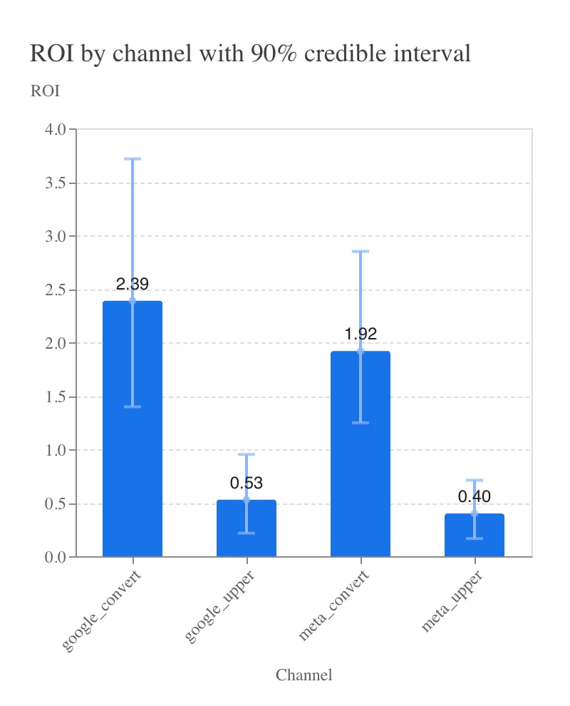
Present the results as ranges. Two questions usually come up the first time. "Why is the uncertainty so wide?" It was always there; a single figure just didn't show it. "What do we do with ranges?" Act on the numbers whose ranges are narrow, and test the ones that aren't. Step 8 turns that into a rule for budget moves.
Step 8: budget scenarios
optimisation:
  start: "2024-11-04"
  end: "2024-12-23"                 # the last WEEK START in the period
  spend_bound: 0.3                   # each channel may move ±30% from its share
  budget_multipliers: [0.8, 1.0, 1.2]
Meridian's optimiser re-splits a budget to maximise incremental revenue within those bounds, and the bounds matter: recommendations far outside the spend the model has seen are guesses. It works over weeks it has observed, so last year's peak flighting stands in for this year's.
Read the peak on its own. At peak spend every channel is deep in diminishing returns, and that's where the average return and the return on the next pound part company:
The optimiser maximises the expected (posterior mean) incremental revenue, which says nothing about how sure the gain is. So the toolkit scores the current split and the new one again on every posterior draw, the way the optimiser scores them. On the synthetic brand, re-splitting last year's Christmas budget within ±30% adds 6.6% to its incremental revenue on average; the new split wins in every draw, and in nine draws out of ten it adds at least 4.2%. The rule I use: move budget when the new split wins in at least 80% of draws, and test it first when it doesn't. The readout applies it to every scenario.
The same draws price the budget level. Adding 20% to the peak budget brings back about 35p per extra £1 (27p to 45p across the middle 80% of draws), far short of the £2 a 50% margin needs. So the bigger decision is often how much to spend, not where.
Step 9: the Scenario Planner
Meridian's Scenario Planner (in open beta) is a report in Data Studio (called Looker Studio until April 2026) on top of a Google Sheet. People pick a period and a budget, and it shows the recommended split and each channel's response curve, so the team can try their own budgets instead of asking for another analysis.
- A person owns the sheet. Service accounts can't own Drive files, so create an empty sheet as the person who should own the report and share it with the service account as Editor.
- Put its id in the config (
planner.spreadsheet_id) and run the chain once:sync, thenorchestrate. - Open the report link once as the owner and click Edit and save. If you're signed in to several Google accounts, check the link opens under the owner.
- Refreshes rewrite the same sheet in place, keeping its tabs, so the saved report updates itself. Large tables are written in chunks, and empty or infinite values are cleaned first.
Two gotchas. The connector rejects a bare /d/<id> sheet URL; it needs the /edit form. And the planner opens on different defaults (the whole period, each channel from -50% to +100%) than the optimisation reports, so set expectations or demo it live.
Step 10: run it in the cloud, every quarter
Cloud runs use Vertex AI Colab Enterprise: the same notebook, run as a job in your project, as a service account. More cores barely help and a GPU isn't needed, so run fits side by side instead. The service account needs:
- Colab Enterprise User on the project, to start runs, including the orchestrator starting child fits.
- BigQuery Job User and Data Viewer, to read the input view and the tables behind it.
- Storage Object Admin and Legacy Bucket Reader on the output bucket. Colab needs
storage.buckets.getto save the executed notebook, and Object Admin doesn't include it. - Service Account User and Token Creator on itself, so the orchestrator can launch fits as the same account and mint a Sheets-scoped token for the planner (runtime tokens carry the cloud-platform scope only).
Colab Enterprise fails a run that would go over quota rather than waiting, and three quotas bite: all-region CPUs (often 32 on a young project, so three 8-core fits at once), external IP addresses per region (one per runtime), and regional SSD, because every runtime takes a boot disk of about 100 GB on SSD whatever disk type its template sets.
python3 mmm/run_mmm.py --config brand/mmm.yaml sync        # after any change to code or config
python3 mmm/run_mmm.py --config brand/mmm.yaml orchestrate # fits, planner tables, sheet
python3 mmm/run_mmm.py --config brand/mmm.yaml schedule    # once: 06:00 on 7 Jan / Apr / Jul / Oct
The schedule runs an orchestrator notebook that fits the refresh grid (the main fit plus the three holdouts), builds the planner tables from the main fit and rewrites the sheet, with nobody involved. Run a changed specification as a named challenger alongside the main fit rather than replacing it silently.
What a good MMM engagement looks like
Prerequisites: enough weekly data across all major channels, including non-digital where relevant: Google's rule of thumb is two years for a model by market and three for a national one. On a warehouse that already holds the data, the build takes days; without one, data preparation is most of the work.
Deliverables: the model, with its priors and their sources, diagnostics, posteriors and response curves; an assumptions register of every judgement call, gone through with the client before any number is presented; Meridian's reports and the Scenario Planner; a readout that leads with what held across the sensitivity grid, quotes the rest as ranges and gives every budget change its chance of beating the current split; and a test plan.
Tests: the weakest numbers become experiments, and each result goes back into the next fit through experiments.csv (step 3). Meridian discounts a test that's small, short or old, so plan each one to count, and size it before proposing it. A brand on/off test for PMax, switching a brand negative keyword list on and off by day at random for about eight weeks in one large market, can detect a move of around 15% in orders; comparing two markets that peak at different times of year usually can't. A video geo holdout and a Meta Conversion Lift test cover the upper funnel and Meta's conversion campaigns.
Cadence: a quarterly refit on the schedule, and an interim refit when a test reads or something significant changes (a new channel, a new market, a major creative pivot).
MMM doesn't replace the signal layer in L/003 and L/004; the two do different jobs. Clean platform signal keeps the day-to-day bidding working, and the model shows where the next pound of budget should go.
The toolkit is free to use and adapt. If you'd rather have the whole workflow built for you, from the data and the checks to the budget recommendation, get in touch.